Next, XLS Trader offers four sets of functions calling order logs detailing trading activity of the trade system:
•=AllOrdersLog()
•=FilledOrdersLog()
•=WorkingOrdersLog()
•=FailedOrdersLog()
The AllOrdersLog will display all orders working, filled, canceled and failed (rejected). The FilledOrdersLog displays just filled orders. The WorkingOrdersLog displays just working orders and the FailedOrdersLog displays orders that failed to be accepted by the exchange but passed CQG's gateway.
Two key factors about using the Order Log functions: 1) These functions have to be entered as arrays in Excel, and 2) these functions do not save the data. If you log out of the trading system then the next time you log in the Logs are created from the new log in time. You cannot retrieve previous order log information.
To use the AllOrdersLog function you first decide just how many rows in Excel you want to dedicate for calling the log data. You may want to use this function off to the side of your main work so there is plenty of room for displaying the log data.
The function requires the cell reference for the Trade System. In our example, the Trade System function is cell C2.
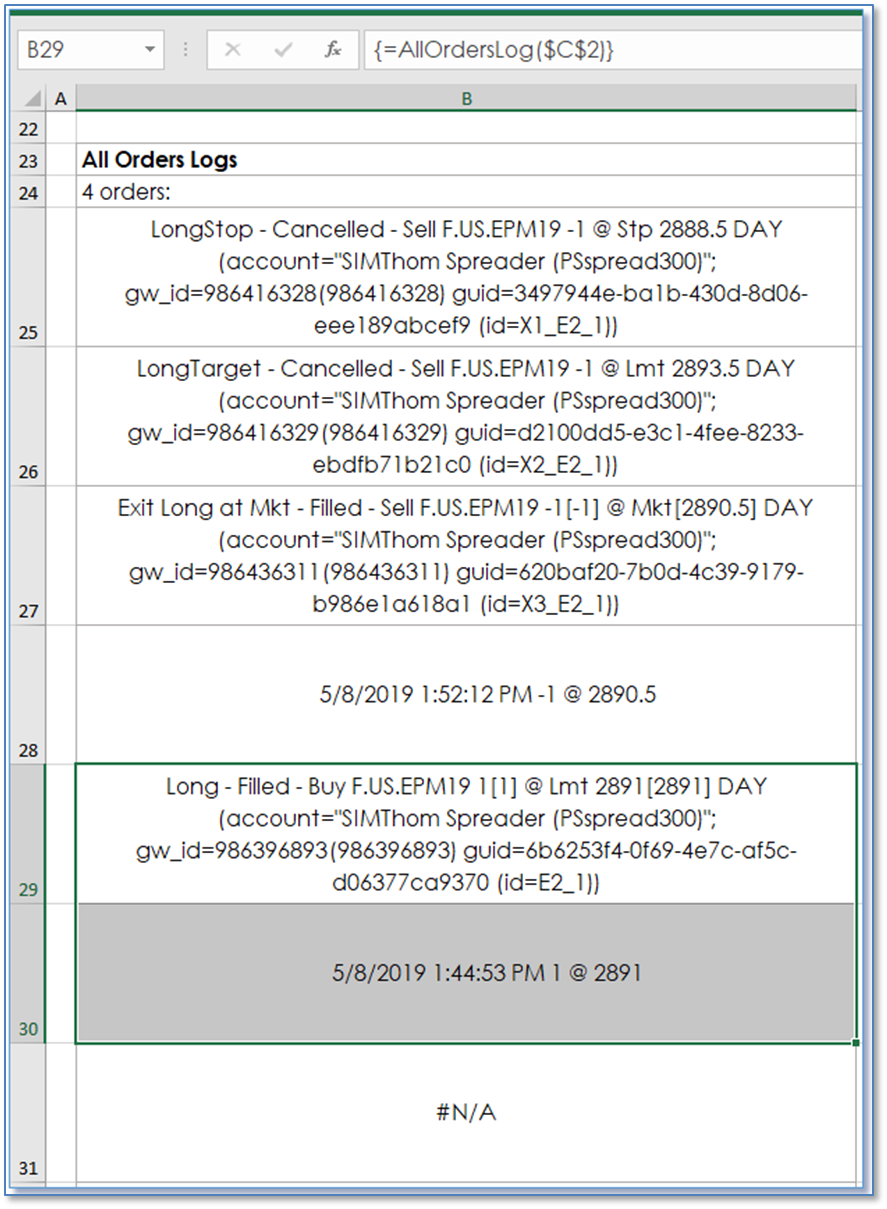
To enter the functions to return an array you select the rows you want to display the log data and in the first row’s formula box then enter =AllOrdersLog($C$2) and then hit the key combination Shift+Ctrl+Enter.
The result should be the selected section will display {=AllOrdersLog($C$2)}. The curly brackets indicate this is an array. You will initially see the #N/A error as there is no log data, yet.
Once orders are placed and executed, you will see similar information as shown below. The first order is at the bottom. It was a “Long” order, which was filled. Cell B30 shows the date, time, quantity and price. Cell B29 shows more details pertaining to the actual order. A target order and a stop loss order was also placed.
Then the long position was liquidated using a market order. You see the date, time, quantity and price when the market order was executed and that the target and stop orders were canceled.
There is quite a bit of information delivered using the Order Logs functions. You may not be interested in seeing this much detail and want to better manage the space in Excel.
The function below is looking at the log data that is on the tab named Model and cell B25. The function finds the first open parenthesis and cuts off everything including the space ahead of the open parenthesis. You copy and paste this formula down in the column you want to see the filtered information. You will need to change it to access the first row cell reference, such as B1.
=IFERROR(LEFT(Model!B25,FIND("~",SUBSTITUTE(Model!B25,"(","~",1))-1),Model!B25)
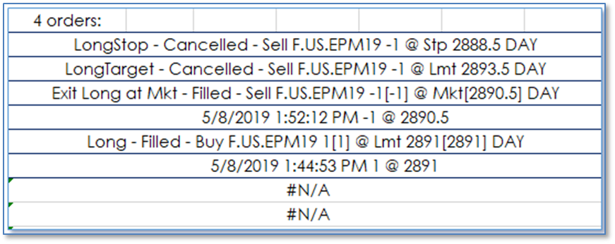
The FilledOrdersLog, WorkingOrdersLog and the FailedOrdersLog displays the data in the same fashion as the AllOrdersLogs.
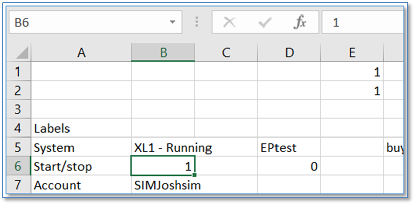
A tip: Notice in the screen capture of the AllOrdersLog the data fits in the cell. You will find almost immediately that many XLS Trader functions display more information than within the default cell width. For instance, the TradeSystem() function appends the string “ – Running” to the cell output when successfully started. Below is a workbook before the trade system is started:
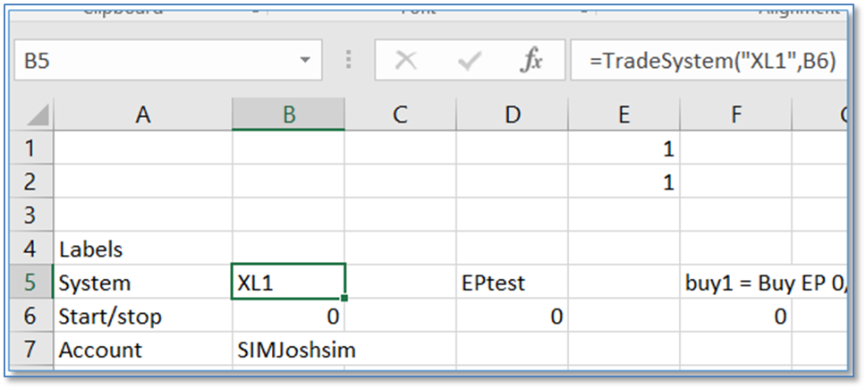
When we turn this system on using it’s trigger in cell B6, we see the display spills over into C5:
When creating entries, this issue is even more pronounced:
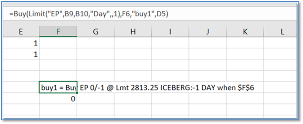
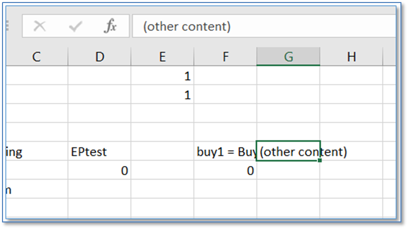
The full formula runs over the cells to the right. This may not be an issue if there is no content in the cells to the right of the functions, but otherwise that content would be chopped off like below:
If you want to be able to see all of this information, there are two options: 1) expand the column width for that cell (and all other cells above and below it), or 2) format the cell to allow the text to wrap down in multiple rows of text.
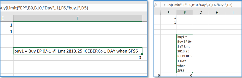
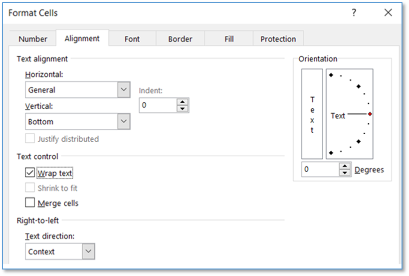
In order to implement the text wrap formatting, select the cell(s) you want to apply this to, or the “select all cells” button in the top left corner at the intersection of the column and row headers, choose “Format Cells …”, and in the window that opens, select the “Alignment” tab. You will see a checkbox for “Wrap text.” Once checked, the text will not run over into adjacent cells.